实验代码参考: Interpretability: LIME and SHAP in prose and code
前期准备
实验数据集(Kaggle: Telco Customer Churn)
运行商用户流失预测:字段0~19是用户属性,字段20为标签(Churn: True 表示客户流失)。
Available features:  ['gender', 'SeniorCitizen', 'Partner', 'Dependents', 'tenure', 'PhoneService', 'MultipleLines', 'InternetService', 'OnlineSecurity', 'OnlineBackup', 'DeviceProtection', 'TechSupport', 'StreamingTV', 'StreamingMovies', 'Contract', 'PaperlessBilling', 'PaymentMethod', 'MonthlyCharges', 'TotalCharges']

Label Balance - [No Churn, Churn] :  [5163, 1869]
数据集包含 7,043 个用户,其中约 25% 的为流失用户。每个用户的 20 个特征中包含用户的固有属性(gender 性别、SeniorCitizen 是否老年人、Partner 是否单身 等),以及描述开通服务(PhoneService 电话业务、MultipleLines 多线业务、InternetService 网络服务 等)、用户账户(Contract 合同方式、PaperlessBilling 电子账单、MonthlyCharges 月费用 等)的信息。
- 数据集的特征中即包含连续数据,又包含类别数据;
- 根据模型的类型,可以将类别字段用不同的方法表示。例如,基于树的模型可以直接使用类别编码来训练,而其他模型(线性回归、神经网络等)使用独热编码的类别变量会取得更好的效果。
训练模型(NB, LR, DT, RF, GBT, MLP)
from sklearn.tree import DecisionTreeClassifier
from sklearn.ensemble import RandomForestClassifier
from sklearn.ensemble import GradientBoostingClassifier
from sklearn.naive_bayes import GaussianNB
from sklearn.neural_network import MLPClassifier
from sklearn.svm import SVC
from sklearn.linear_model import LogisticRegressionCV

trained_models = [] #  keep track of all details for models we train
def train_model(model, data, labels):
  X = data
  y = labels.values
  X_train, X_test, y_train, y_test = train_test_split(X, y, random_state=42)

  pipe = Pipeline([('scaler', StandardScaler()),('clf', model["clf"])])
  start_time = time.time()
  pipe.fit(X_train, y_train)
  train_time = time.time() - start_time

  train_accuracy =  pipe.score(X_train, y_train)
  test_accuracy = pipe.score(X_test, y_test)
  model_details = {"name": model["name"], "train_accuracy":train_accuracy, "test_accuracy":test_accuracy, "train_time": train_time, "model": pipe}
  return model_details

models = [
          {"name": "Naive Bayes", "clf": GaussianNB()},
          {"name": "logistic regression", "clf": LogisticRegressionCV()},
          {"name": "Decision Tree", "clf": DecisionTreeClassifier()},
          {"name": "Random Forest", "clf": RandomForestClassifier(n_estimators=100)},
          {"name": "Gradient Boosting", "clf": GradientBoostingClassifier(n_estimators=100)},
          {"name": "MLP Classifier", "clf": MLPClassifier(solver='adam', alpha=1e-1, hidden_layer_sizes=(10,10,5,2), max_iter=500, random_state=42)}]

for model in models:
  model_details = train_model(model, current_data, labels)
  trained_models.append(model_details)
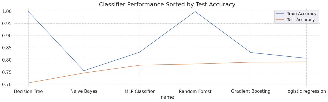
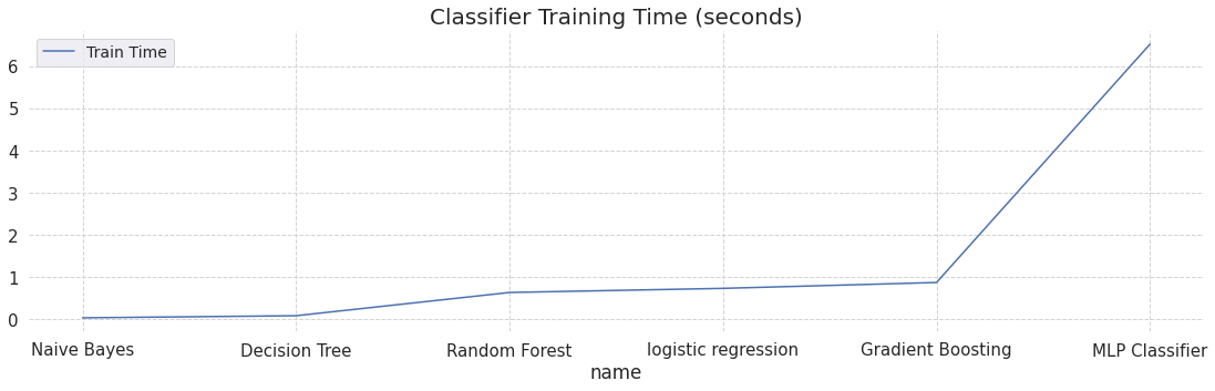
训练好的6个模型信息以字典的形式存在列表 trained_models 中,模型存储在其对应字典的 model 字段。各个模型的测试准确率和训练时间如下图所示。
解释简单模型(Global+Intrinsic, White-box)
"""
画图,其中seaborn基于matplotlib
"""
import matplotlib.pyplot as plt
import seaborn as sns
Logistic Regression Coefficients
"""
current_data.columns -> feature_names
"""
plt.figure(figsize=(15,6))
color_list =  sns.color_palette("dark", len(feature_names))
top_x = 20
logistic_reg_coeff = trained_models[1]["model"]["clf"].coef_[0]
idx = np.argsort(np.abs(logistic_reg_coeff))[::-1]
lreg_ax = plt.barh(feature_names[idx[:top_x]][::-1], logistic_reg_coeff[idx[:top_x]][::-1])
for i,bar in enumerate(lreg_ax):
  bar.set_color(color_list[idx[:top_x][::-1][i]])
  plt.box(False)
lr_title = plt.suptitle("Logistic Regression. Top " + str(top_x) + " Coefficients.", fontsize=20, fontweight="normal")
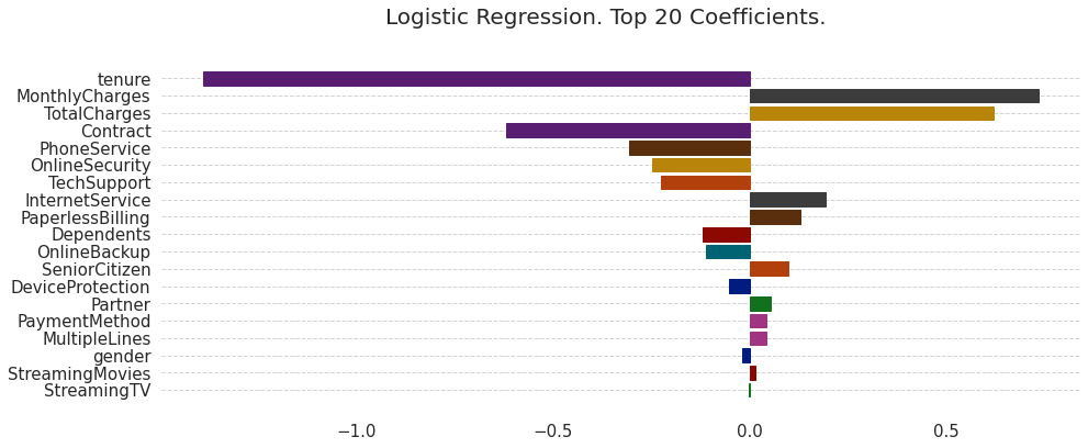
-
how an increase/change in each feature might result in a change in the log odds that the customer will churn.
-
a general understanding of how important a feature is for the entire dataset.
Feature Importance Scores (Tree-based Models: DT, RF, GBT)
决策树特征重要性
sklearn 中的决策树默认的属性划分使用 CART 算法,每个节点有对应的 gini index (值越小,误分错误率越低,纯度越高)。
Feature Importance = 特征权重 * (当前节点的 Impurity - 子节点 Impurity 的加权和)
即 $N_t / N * (impurity - N_{t_R} / N_t * impurity_R - N_{t_L} / N_t * impurity_L)$,
其中 $N$ 是样本总数, $N_t$ 是当前节点样本数,$N_{t_R}$ 是右子节点的样本数, $N_{t_L}$ 是左子节点的样本数;
impurity 直译为不纯度,可以使用基尼指数或信息熵来衡量。以基尼指数的实现为例,假设有样本
X = [[1,0,0], [0,0,0], [0,0,1], [0,1,0]]
y = [1,0,1,1]
使用sklearn训练并可视化模型:
from sklearn.tree import export_graphviz

model=DecisionTreeClassifier() # max_depth=3
model.fit(X, y)
export_graphviz(model, out_file=open('tree.dot','w'), feature_names=['x[0]','x[1]','x[2]'],class_names=['0','1'],rounded=True, filled=True)

"""
Convert .dot to .png
    dot -Tpng tree.dot -o tree.png
"""
import os
os.system("dot -Tpng tree.dot -o tree.png")
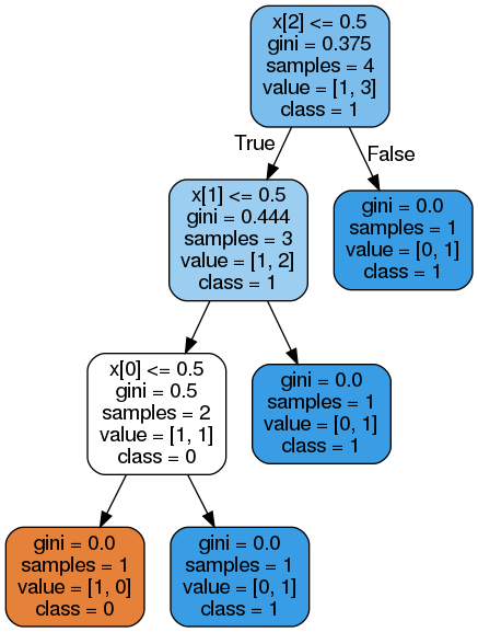
则特征 x[0],x[1],x[2] 的 feature importance 计算方法如下:
fi_0 = (2 / 4) * (0.5) # 0.25
fi_1 = (3 / 4) * (0.444 - (2 / 3 * 0.5)) # 0.083
fi_2 = (4 / 4) * (0.375 - (3 / 4 * 0.444)) # 0.042
# 要使所有特征重要性的和为1,则可以进行L1归一化
from sklearn import preprocessing
preprocessing.normalize([[fi_0,fi_1,fi_2]], norm='l1') # array([[0.66666667, 0.22133333, 0.112     ]])
可以验证该结果与 model.feature_importances_ 是一致的([0.66666667 0.22222222 0.11111111])。
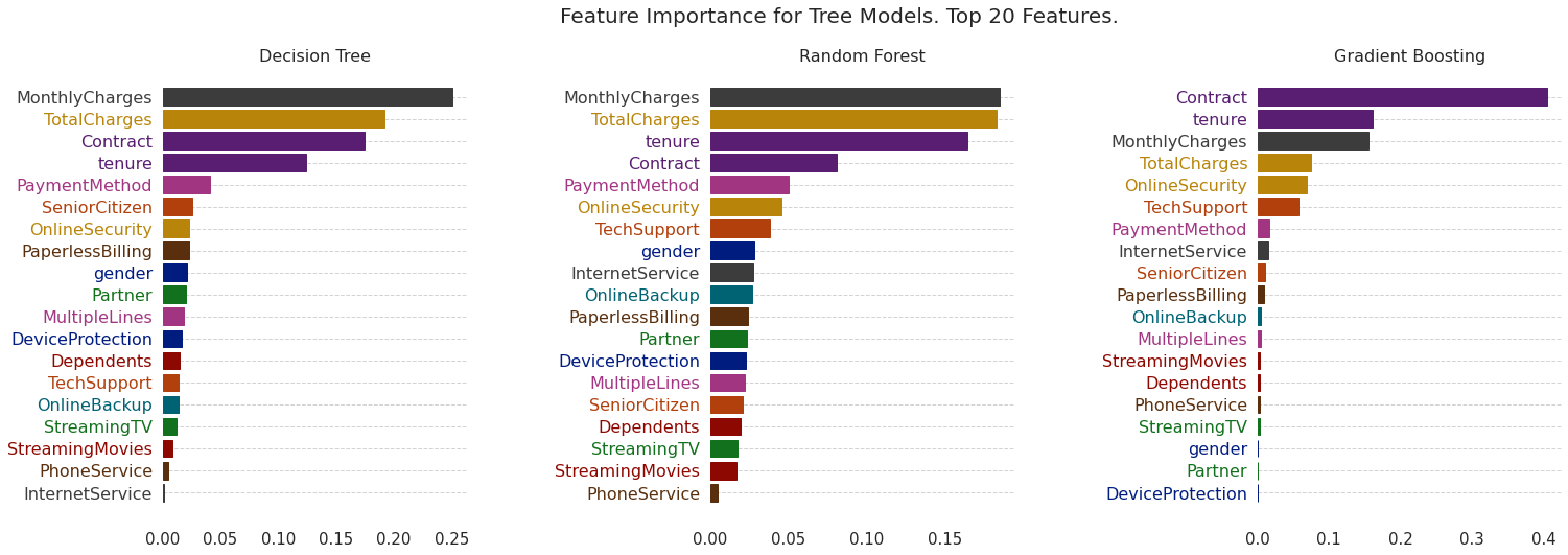
可视化解释树模型
回到用户流失预测的例子,可视化代码如下:
tree_models = []
setup_plot()
color_list =  sns.color_palette("dark", len(current_data.columns))
top_x = 20 # number of x most important features to show
for model in trained_models:
  if hasattr(model["model"]["clf"], 'feature_importances_'):
    tree_models.append({"name":model["name"], "fi": model["model"]["clf"].feature_importances_})


fig, axs = plt.subplots(1,3, figsize=(24, 8), facecolor='w', edgecolor='k')
fig.subplots_adjust(hspace = 0.5, wspace=0.8)
axs = axs.ravel()
for i in range(len(tree_models)):
  feature_importance = tree_models[i]["fi"]
  indices = np.argsort(feature_importance)
  indices = indices[-top_x:]

  bars = axs[i].barh(range(len(indices)), feature_importance[indices], color='b', align='center')
  axs[i].set_title( tree_models[i]["name"], fontweight="normal", fontsize=16)

  plt.sca(axs[i])
  plt.yticks(range(len(indices)), [current_data.columns[j] for j in indices], fontweight="normal", fontsize=16)

  # print(len(plt.gca().get_yticklabels()), len(indices))
  for i, ticklabel in enumerate(plt.gca().get_yticklabels()):
    ticklabel.set_color(color_list[indices[i]])

  for i,bar in enumerate(bars):
    bar.set_color(color_list[indices[i]])
  plt.box(False)

plt.suptitle("Feature Importance for Tree Models. Top " + str(top_x) + " Features.", fontsize=20, fontweight="normal")
解释任意模型 (Local+Posthoc, Black-box)
Local Interpretable Model-agnostic Explanation(LIME)
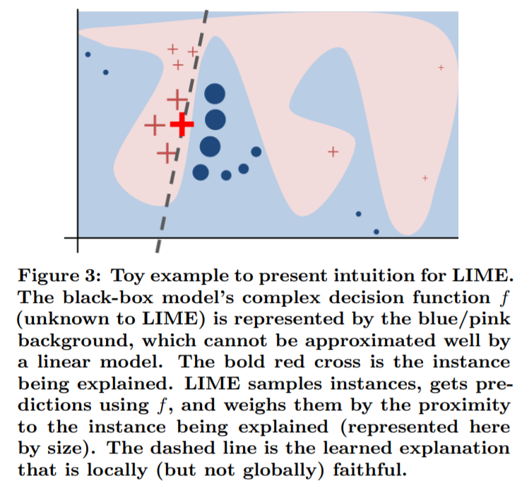
原理
KDD’16, Why Should I Trust You? Explaining the Predictions of Any Classifier
目标:找到一个自身可解释的模型 $g$ (如线性模型) 近似 $f$,使得 $\mathcal{L}(f,g,\pi_x)$ 最小。损失函数
\[\mathcal L = \sum_{i=1}^{l}\pi_x(\widetilde{x}_i)(f_N(\widetilde{x}_i)-g(\widetilde{x}_i))^2\]度量的是在 $\pi_x$ 定义的邻域里 $g$ 近似 $f$ 的非保真度。
a measure of how unfaithful $g$ is in approximating $f$ in the locality defined by $\pi_x$
- 样本的表示:original representation $x \in \mathbb R^d$, interpretable representation $x^\prime \in {0,1}^{d^\prime}$;
- 邻域的估计:随机采样 $x^\prime$ 上要保留的非零值,施加的扰动 $z^\prime \in {0,1}^{d^\prime}$,恢复到原表征域 $z \in \mathbb R^d$,得到原模型的预测结果 $f(z)$,作为解释模型的标签;
- 非保真度的度量:加权的均方误差,其中每个扰动的权重是 $z$ 和 $x$ 的相似度(primary intuition 见下图),
- 权重函数定义为 $\pi_x(z)=e^{-\frac{D(x,z)^2}{\sigma^2}}$,其中距离函数 $D$ 对文本可选余弦距离(1-余弦相似度),对图像可选 L2距离。
实现
LIME 库相关接口
Python 库 LIME 提供了实现模型解释的接口,按数据类型分为 表格(LimeTabularExplainer), 图像(LimeImageExplainer) 和 文本(LimeTextExplainer)。对于本实验数据集而言,我们使用LimeTabularExplainer。
from lime.lime_tabular import LimeTabularExplainer
代码实现上对应以下三个步骤:
- 给定一个数据点,随机扰动它的特征。对于 tabular (i.e. matrix) data,数值上加一个小的噪声,类别特征做是否改变的二元选择;
- 得到所有扰动后的数据点的预测结果;
- 使用这些数据点计算一个近似的线性模型,线性模型的系数被用作解释。
class LimeTabularExplainer(object):
    """Explains predictions on tabular (i.e. matrix) data.
    For numerical features, perturb them by sampling from a Normal(0,1) and doing the inverse operation of mean-centering and scaling, according to the means and stds in the training data.
    For categorical features, perturb by sampling according to the training distribution, and making a binary feature that is 1 when the value is the same as the instance being explained."""
创建 LimeTabularExplainer 类
- 必要参数是
training_data,因为采样时会依照训练数据的分布,类型是 numpy 二维数组; feature_names和class_names分别是特征和类别的名字(字符串);- 由于类别数据和数值数据的处理方式不同,需要把对应的特征编号传入参数
categorical_features中; mode参数代表任务的类型,可选分类(classification)或回归(regression)。
解释单个样本:调用该类的 explain_instance 方法,返回 Explanation 对象
- 必要参数
data_row:待解释的样本(一维 numpy 数组); - 必要参数
predict_fn,用于预测的函数(对分类任务而言,输入 numpy 数组,输出预测概率值,例如 sklearn 的分类器的predict_proba); num_features表示解释结果中最多能呈现的特征数量;distance_metric默认的是euclidean。
返回的 Explanation 有
as_map方法:返回字典类型,标签 -> 元组(特征id,权重)的列表local_pred属性:字典类型,类别标签 -> 概率
调用接口实现模型解释
lime_data_explainations
lime_metrics
lime_explanation_time
from lime.lime_tabular import LimeTabularExplainer

def get_lime_explainer(model, data, labels):
  cat_feat_ix = [i for i,c in enumerate(data.columns) if pd.api.types.is_categorical_dtype(data[c])]
  feat_names = list(data.columns)
  class_names = list(labels.unique())
  scaler = model["model"]["scaler"]
  data = scaler.transform(data) # scale data to reflect train time scaling
  lime_explainer = LimeTabularExplainer(data,
                                      feature_names=feat_names,
                                      class_names=class_names,
                                      categorical_features=cat_feat_ix ,
                                      mode="classification"
                                      )
  return lime_explainer

def lime_explain(explainer, data, predict_method, num_features):
  explanation = explainer.explain_instance(data, predict_method, num_features=num_features)
  return explanation

# ==========================
lime_data_explainations = []
lime_metrics = []
lime_explanation_time = []
feat_names = list(current_data.columns)
test_data_index = 6
for current_model in trained_models:
  scaler = current_model["model"]["scaler"]
  scaled_test_data = scaler.transform(X_test)
  predict_method = current_model["model"]["clf"].predict_proba

  start_time = time.time()
  # explain first sample from test data
  lime_explainer = get_lime_explainer(current_model, X_train, y_train)
  explanation = lime_explain(lime_explainer, scaled_test_data[test_data_index], predict_method, top_x)
  elapsed_time = time.time() - start_time

  ex_holder = {}
  for feat_index,ex in explanation.as_map()[1] :
    ex_holder[feat_names[feat_index]] = ex

  lime_data_explainations.append(ex_holder)
  actual_pred = predict_method(scaled_test_data[test_data_index].reshape(1,-1))
  perc_pred_diff =  abs(actual_pred[0][1] - explanation.local_pred[0])
  lime_explanation_time.append({"time": elapsed_time, "model": current_model["name"] })
  lime_metrics.append({"lime class1": explanation.local_pred[0], "actual class1": actual_pred[0][1], "class_diff": round(perc_pred_diff,3), "model": current_model["name"] })
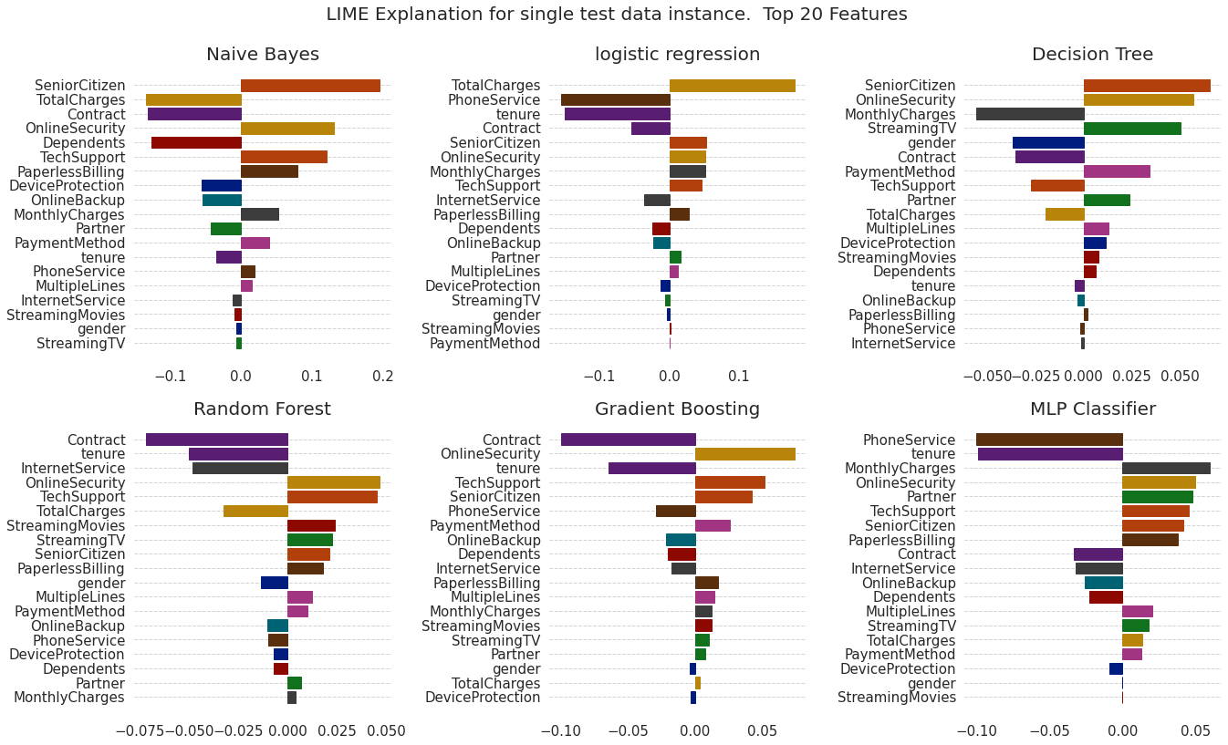
可视化解释结果
def plot_lime_exp(fig, fig_index, exp_data, title):
  features =  list(exp_data.keys())[::-1]
  explanations = list(exp_data.values())[::-1]
  ax = fig.add_subplot(fig_index)
  lime_bar = ax.barh( features, explanations )
  ax.set_title(title, fontsize = 20)
  for i,bar in enumerate(lime_bar):
    bar.set_color(color_list[list(current_data.columns).index(features[i])])
    plt.box(False)
fig = plt.figure(figsize=(19,12))

# Plot lime explanations for trained models
for i, dex in enumerate(lime_data_explainations):
  fig_index = "23" + str(i+1)
  plot_lime_exp(fig, fig_index, lime_data_explainations[i], trained_models[i]["name"])

plt.suptitle( " LIME Explanation for single test data instance.  Top " + str(top_x) + " Features", fontsize=20, fontweight="normal")
fig.tight_layout(rect=[0, 0.03, 1, 0.95])

# Plot run time for explanations
lx_df = pd.DataFrame(lime_explanation_time)
lx_df.sort_values("time", inplace=True)
setup_plot()
lx_ax = lx_df.plot(kind="line", x="model", title="Runtime (seconds) for single test data instance LIME explanation", figsize=(22,6))
lx_ax.title.set_size(20)
lx_ax.legend(["Run time"])
plt.box(False)
SHapley Additive exPlanations(SHAP)
原理
NIPS’17, A Unified Approach to Interpreting Model Predictions
将包含 LIME, DeepLIFT 在内的方法统一为 additive feature attribution methods,提出 SHAP values 应用到这一类方法上,作为有唯一解的特征重要性。
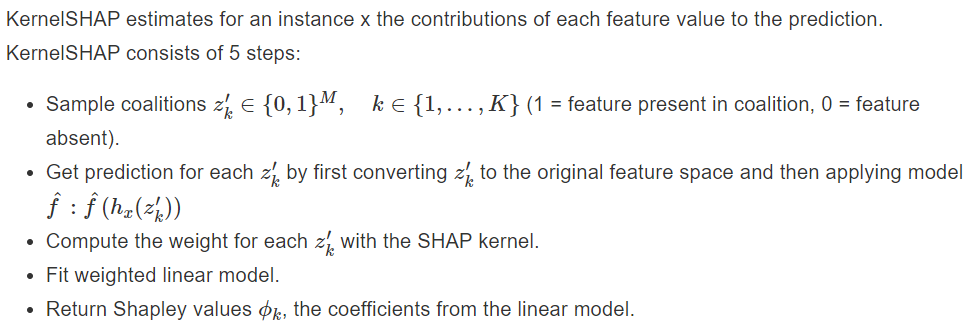
这里介绍与模型无关的 Kernel SHAP(Linear LIME + Shapley values),损失函数为 $L(f,g,\pi_{x^\prime}) = \sum_{z^{\prime}\in\mathcal Z} [f(h_x^{-1}(z^\prime))-g(z^\prime)]^2\pi_{x^\prime}(z^\prime)$
- 将输出值归因到每一个特征的 shapely 值上,因此简化的可解释模型 $g$ 表示为二元变量的线性函数 $g(z^\prime)=\phi_0 + \sum_{j=1}^{M} \phi_jz_j^\prime$,
- 其中 $\phi_i$ 是要求的 shapely 值,$\phi_0$ 代表(训练样本输出结果的)平均值。
- 权重函数 $\pi$ 为 $\pi_{x^\prime}(z^{\prime})=\frac{1}{C_M^{\vert z^{\prime} \vert} }\frac{M-1}{\vert z^{\prime} \vert (M - \vert z^{\prime} \vert)}$,
- 其中 $M$ 是 $x^\prime$ 的维数, $\vert z^{\prime} \vert$ 是 $z^\prime$ 中非零值的个数;
- $\vert z^{\prime} \vert \in (0, M)$,共 $M-1$ 种取值(不包含边界值,否则权重为正无穷),因此右项的范围是 $(0,1]$;
- 若有很多 1 或很多 0 则取较高的权重,若 0 和 1 数量相近则取较低的权重。
实现时的 5 个步骤
与LIME的联系与区别
| SHAP | LIME | |
|---|---|---|
| $x^\prime$ 含义的表述 | simplified features | interpretable representation |
| $x^\prime$ 维度的记法 | $M$ | $d^\prime$ |
| 线性模型 $g^\prime$ | 非齐次,含义是特征的沙普利值加和 | 齐次(无常数项) |
| 权重函数 $\pi$ | 扰动对估算特征边际贡献的作用 | 扰动样本 $z$ 与原样本 $x$ 的相似性 |

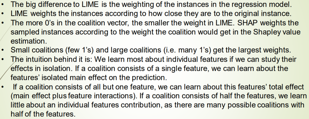
SHAP中距离的计算根据Simplified Features中0的数量, 若有很多0或是很多1, 他的权重都是比较高的,这是因为
- 若都是0, 只有一个是1, 那么我们可以很好的计算出那个是1的特征的贡献.
- 若只有一个是0, 我们可以计算出那个是0的特征的贡献.
- 如果一半是0, 一半是1, 那么会有很多种组合, 就很难计算出每一个特征的贡献
推荐参考:https://mathpretty.com/10699.html
实现
SHAP Library: https://shap.readthedocs.io/en/latest
其中Kernel SHAP在实现时分为两种情况:特征空间 $M$ 较小时遍历整个采样空间 $2^M$,较大时则使用采样的方法近似。
import shap
shap.initjs() # 用来显示的

""" 新建一个解释器
	这里传入两个变量, 1. 模型; 2. 训练数据
"""
explainer = shap.KernelExplainer(batch_predict, x)

print(explainer.expected_value) # 输出是各类别概率的平均值
使用 KernelExplainer 的 shap_values 方法计算单个数据(x[0])特征的沙普利值:
shap_values = explainer.shap_values(x[0])
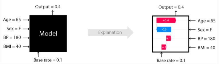
解释该样本在 current_label 类别对应概率的输出值 -> 使用force_plot方法,传入类别对应的 base rate 以及样本特征的沙普利值,将解释结果可视化(若要指定特征名字则使用 feature_names 参数):
shap.force_plot(base_value=explainer.expected_value[current_label],
                shap_values=shap_values[current_label],
                features=x[0])

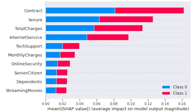
解释一组样本在某类上的输出 -> 使用summary_plot方法,传入 shap_values 和 features 参数(参见文档)。