PyG框架的图数据

Contents

torchgeometric.data
以ENZYMES数据集示例Batch
自定义数据集
- Creating “In Memory Datasets”
- Creating “Larger” Datasets
NeighborSampler的使用

PyTorch Geometric (PyG) is a geometric deep learning extension library for PyTorch.

torch_geometric.data

共以下十个类：

单（个/批）图数据：
- Data: A plain old python object modeling a single graph with various (optional) attributes
- Batch: A plain old python object modeling a batch of graphs as one big (dicconnected) graph.
  - With torch_geometric.data.Data being the base class, all its methods can also be used here.
  - In addition, single graphs can be reconstructed via the assignment vector batch, which maps each node to its respective graph identifier.
为数据集创建提供的两个抽象类（官方教程）：
- Dataset: Dataset base class for creating graph datasets.
- InMemoryDataset: … fit completely into memory. （ torch_geometric.datasets 中的现有数据集多从此类继承）

数据集分批载入：
- DataLoader: Data loader which merges data objects from a torch_geometric.data.dataset to a mini-batch.
- DataListLoader: 和DataLoader的唯一区别就是返回的不是Batch而是data组成的list；
- DenseDataLoader: All graphs in the dataset needs to have the same shape for each its attributes.
- ClusterLoader: Clusters/partitions a graph data object into multiple subgraphs, as motivated by the “Cluster-GCN: An Efficient Algorithm for Training Deep and Large Graph Convolutional Networks” paper.
子图采样（来自两篇论文）：
- NeighborSampler: The neighbor sampler from the “Inductive Representation Learning on Large Graphs” paper which iterates over graph nodes in a mini-batch fashion and constructs sampled subgraphs of size num_hops.
- ClusterData: Clusters/partitions a graph data object into multiple subgraphs, as motivated by the “Cluster-GCN: An Efficient Algorithm for Training Deep and Large Graph Convolutional Networks” paper.

以ENZYMES数据集示例Batch

ENZYMES is a dataset of protein tertiary structures obtained from (Borgwardt et al., 2005) consisting of 600 enzymes from the BRENDA enzyme database (Schomburg et al., 2004). In this case the task is to correctly assign each enzyme to one of the 6 EC top-level classes.

以用于图分类的ENZYMES数据集（包含有600个graphs，6个类别）为例：

# node_labels: (0,1,2); node_attr: 18 => node_features: 21
dataset = TUDataset(root='/tmp/ENZYMES', name='ENZYMES', use_node_attr=True)

print(dataset[0].keys)

>>> ['x', 'edge_index', 'y']

loader = DataLoader(dataset, batch_size=64, shuffle=True)
for batch in loader:
    print(batch)
    
>>> # 共 64*9+24=600 个graphs
    Batch(batch=[1979], edge_index=[2, 7754], x=[1979, 21], y=[64])
    Batch(batch=[2103], edge_index=[2, 8178], x=[2103, 21], y=[64])
    Batch(batch=[2350], edge_index=[2, 8956], x=[2350, 21], y=[64])
    Batch(batch=[2051], edge_index=[2, 7770], x=[2051, 21], y=[64])
    Batch(batch=[1949], edge_index=[2, 7362], x=[1949, 21], y=[64])
    Batch(batch=[1944], edge_index=[2, 7668], x=[1944, 21], y=[64])
    Batch(batch=[2227], edge_index=[2, 8320], x=[2227, 21], y=[64])
    Batch(batch=[2162], edge_index=[2, 7800], x=[2162, 21], y=[64])
    Batch(batch=[2133], edge_index=[2, 8162], x=[2133, 21], y=[64])
    Batch(batch=[682], edge_index=[2, 2594], x=[682, 21], y=[24])

关于此数据集Batch的属性说明如下：

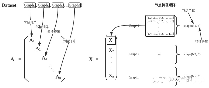
edge_index：连接边的source和target节点
x：整个batch的节点特征矩阵
y：graph标签
batch：列向量，用于指示每个节点属于batch中的第几个graph

PyG通过创建一个稀疏的块对角矩阵来实现并行化操作。
下图引自《番外篇：PyG框架及Cora数据集简介》。

自定义数据集

Creating “In Memory Datasets”

必须实现的四个方法:

torch_geometric.data.InMemoryDataset.raw_file_names():

A list of files in the raw_dir which needs to be found in order to skip the download.
torch_geometric.data.InMemoryDataset.processed_file_names():

A list of files in the processed_dir which needs to be found in order to skip the processing.
torch_geometric.data.InMemoryDataset.download():

Downloads raw data into raw_dir.
torch_geometric.data.InMemoryDataset.process():

Processes raw data and saves it into the processed_dir.

下面实现一个MyOwnDatasetTest类：

import torch
from torch_geometric.data import Data

from torch_geometric.data import DataLoader

import torch
from torch_geometric.data import InMemoryDataset


class MyOwnDatasetTest(InMemoryDataset):
    def __init__(self, root, transform=None, pre_transform=None):
        super(MyOwnDatasetTest, self).__init__(root, transform, pre_transform)
        self.data, self.slices = torch.load(self.processed_paths[0])

    @property
    def raw_file_names(self):
        return ['some_file_1', 'some_file_2']
        # pass

    @property
    def processed_file_names(self):
        return ['data.pt']

    def download(self):
        # Download to `self.raw_dir`.
        pass

    def process(self):
        # Read data into huge `Data` list.
        edge_index = torch.tensor([[0, 1],
                                   [1,2]
                                   ], dtype=torch.long)
        y1 = torch.tensor([0], dtype=torch.long)
        y2 = torch.tensor([1], dtype=torch.long)

        data1 = Data(edge_index=edge_index.t().contiguous(), y=y1)
        data2 = Data(edge_index=edge_index.t().contiguous(), y=y2)

        data_list = [data1, data2, data1]

        if self.pre_filter is not None:
            data_list = [data for data in data_list if self.pre_filter(data)]

        if self.pre_transform is not None:
            data_list = [self.pre_transform(data) for data in data_list]

        data, slices = self.collate(data_list)
        print(data,slices)
        torch.save((data, slices), self.processed_paths[0])

测试 MyOwnDatasetTest 类：

dataset = MyOwnDatasetTest(root="./MyOwnDatasetTest")
>>>	# 生成了MyOwnDatasetTest文件夹，其下包含raw和processed两个文件夹
Processing...
Data(edge_index=[2, 6], y=[3]) {'edge_index': tensor([0, 2, 4, 6]), 'y': tensor([0, 1, 2, 3])}
Done!

loader = DataLoader(dataset, batch_size=2, shuffle=True)
for i in loader:
    for k in i.keys:
        print("%s:\t%s"%(k, i[k]))
        print('\n')
>>>
edge_index:	tensor([[0, 1, 3, 4],
        [1, 2, 4, 5]])
y:	tensor([0, 1])
batch:	tensor([0, 0, 0, 1, 1, 1])

edge_index:	tensor([[0, 1],
        [1, 2]])
y:	tensor([0])
batch:	tensor([0, 0, 0])

Creating “Larger” Datasets

进一步再实现两个方法:

torch_geometric.data.Dataset.len():

Returns the number of examples in your dataset.
torch_geometric.data.Dataset.get():

Implements the logic to load a single graph.

跳过下载/处理？不重写 download() 和 process() 方法:

class MyOwnDataset(Dataset):
    def __init__(self, transform=None, pre_transform=None):
        super(MyOwnDataset, self).__init__(None, transform, pre_transform)

并非一定要使用dataset，简单地将 torch_geometric.data.Data 对象的列表传给 torch_geometric.data.DataLoader 类也可以。

e.g., when you want to create synthetic data on the fly without saving them explicitly to disk.

from torch_geometric.data import Data, DataLoader

data_list = [Data(...), ..., Data(...)]
loader = DataLoader(data_list, batch_size=32)

NeighborSampler的使用

依然使用ENZYMES数据集为例：

print(dataset[0].num_nodes)
>>> 16

from torch_geometric.data import NeighborSampler
sampler = NeighborSampler(dataset[0], 1.0, 2, shuffle=True)	# 100%的2跳邻居
for i in sampler.__get_batches__(): # b_id
    print(sampler.__produce_subgraph__(i))
>>> # 16 subgraphs
Data(b_id=[1], e_id=[18], edge_index=[2, 18], n_id=[8], sub_b_id=[1])
Data(b_id=[1], e_id=[27], edge_index=[2, 27], n_id=[12], sub_b_id=[1])
Data(b_id=[1], e_id=[28], edge_index=[2, 28], n_id=[11], sub_b_id=[1])
Data(b_id=[1], e_id=[23], edge_index=[2, 23], n_id=[10], sub_b_id=[1])
Data(b_id=[1], e_id=[10], edge_index=[2, 10], n_id=[7], sub_b_id=[1])
Data(b_id=[1], e_id=[17], edge_index=[2, 17], n_id=[7], sub_b_id=[1])
Data(b_id=[1], e_id=[15], edge_index=[2, 15], n_id=[8], sub_b_id=[1])
Data(b_id=[1], e_id=[20], edge_index=[2, 20], n_id=[10], sub_b_id=[1])
Data(b_id=[1], e_id=[14], edge_index=[2, 14], n_id=[6], sub_b_id=[1])
Data(b_id=[1], e_id=[33], edge_index=[2, 33], n_id=[12], sub_b_id=[1])
Data(b_id=[1], e_id=[23], edge_index=[2, 23], n_id=[10], sub_b_id=[1])
Data(b_id=[1], e_id=[12], edge_index=[2, 12], n_id=[8], sub_b_id=[1])
Data(b_id=[1], e_id=[24], edge_index=[2, 24], n_id=[11], sub_b_id=[1])
Data(b_id=[1], e_id=[16], edge_index=[2, 16], n_id=[10], sub_b_id=[1])
Data(b_id=[1], e_id=[24], edge_index=[2, 24], n_id=[10], sub_b_id=[1])
Data(b_id=[1], e_id=[14], edge_index=[2, 14], n_id=[8], sub_b_id=[1])

查看其中一个子图的Data：

Data(b_id=[1], e_id=[10], edge_index=[2, 10], n_id=[7], sub_b_id=[1])
edge_index: 
tensor([[6, 2, 0, 3, 0, 6, 2, 5, 1, 4],
        [4, 4, 4, 5, 5, 5, 5, 6, 5, 6]])
e_id: 
tensor([19,  1, 49, 35, 48, 18,  0,  4, 38, 21])
n_id: 
tensor([13, 11,  0, 10,  6,  1,  5])
b_id: 
tensor([5])
sub_b_id: 
tensor([6])

b_id: target节点在大图中的序号
e_id: 边在大图中的序号
edge_index: 子图节点序号表示的边连接关系
n_id: 子图中所有点在大图中的序号
b_id: target节点在子图中的序号

PyG框架的图数据

March 17, 2020

torch_geometric.data

以ENZYMES数据集示例Batch

自定义数据集

Creating “In Memory Datasets”

Creating “Larger” Datasets

NeighborSampler的使用

强化学习背景知识

SHAP源码之Masker

SHAP源码之Benchmark示例