SHAP源码之Benchmark示例

Contents

Benchmark XGBoost explanations
Build Explainers
- shap.maskers
- shap.explainers
Run Benchmarks
- shap.benchmark
Visualize Results
- shap.plots.benchmark
  - Show scores across all metrics for all explainers
  - Show detail plots of each metric type

Benchmark XGBoost explanations

These benchmark notebooks compare different types of explainers across a variety of metrics. They are all generated from Jupyter notebooks available on GitHub.

Model: XGBoost
Dataset: Boston Housing (Tabular)

Build Explainers

# use an independent masker
masker = shap.maskers.Independent(X_train)
pmasker = shap.maskers.Partition(X_train)

# build the explainers
explainers = [
    ("Permutation", shap.explainers.Permutation(model.predict, masker)),
    ("Permutation part.", shap.explainers.Permutation(model.predict, pmasker)),
    ("Partition", shap.explainers.Partition(model.predict, pmasker)),
    ("Tree", shap.explainers.Tree(model, masker)),
    ("Tree approx.", shap.explainers.Tree(model, masker, approximate=True)),
    ("Exact", shap.explainers.Exact(model.predict, masker)),
    ("Random", shap.explainers.other.Random(model.predict, masker))
]

shap.maskers

# shap/maskers/__init__.py
from ._masker import Masker
from ._tabular import Independent, Partition, Impute
from ._image import Image
from ._text import Text
from ._fixed import Fixed
from ._composite import Composite
from ._fixed_composite import FixedComposite
from ._output_composite import OutputComposite

The two types of masker used during building the explainers:

masker: Independent masks out tabular features by integrating over the given background dataset.
pmasker: Partition Unlike Independent, Partition respects a hierarchial structure of the data.
- param clustering：string (distance metric to use for creating the clustering of the features) or numpy.ndarray (the clustering of the features).

The following two types of masker are used during benchmarking:

cmasker: Composite merges several maskers for different inputs together into a single composite masker.
Fixed leaves the input unchanged during masking, and is used for things like scoring labels.

shap.explainers

# shap/explainers/__init__.py
from ._permutation import Permutation
from ._partition import Partition
from ._tree import Tree
from ._gpu_tree import GPUTree
from ._exact import Exact
from ._additive import Additive
from ._linear import Linear
from ._sampling import Sampling
from ._deep import Deep

# shap/__init__.py

# explainers
from .explainers._explainer import Explainer
from .explainers._kernel import Kernel as KernelExplainer
from .explainers._sampling import Sampling as SamplingExplainer
from .explainers._tree import Tree as TreeExplainer
from .explainers._gpu_tree import GPUTree as GPUTreeExplainer
from .explainers._deep import Deep as DeepExplainer
from .explainers._gradient import Gradient as GradientExplainer
from .explainers._linear import Linear as LinearExplainer
from .explainers._partition import Partition as PartitionExplainer
from .explainers._permutation import Permutation as PermutationExplainer
from .explainers._additive import Additive as AdditiveExplainer
from .explainers import other # Coefficent, Random, LimeTabular, Maple, TreeMaple, TreeGain

The explainers list is made up of 6 explainers of 4 types (5 classes):

model-agnostic
- “Permutation”, “Permutation part.”: Permutation (masker = masker/pmasker) approximates the Shapley values by iterating through permutations of the inputs.
- “Partition”: Partition has two particularly nice properties
  - model-agnostic but when using a balanced partition tree only has quadradic exact runtime (in term of the number of input features). This is in contrast to the exponential exact runtime of KernalExplainer or SamplingExplainer.
  - always assigns to groups of correlated features the credit that set of features would have had if treated as a group
tree
- “Tree”, “Tree approx.”: Tree (approximate = False/True)
shapley
- “Exact”: Exact computes SHAP values via an optimized exact enumeration.
baseline
- “Random”: Random simply returns random (normally distributed) feature attributions.

Run Benchmarks

# explain with all the explainers
attributions = [(name, exp(X_eval)) for name, exp in explainers] # (str, shap._explanation.Explanation)

results = {} # metric name: shap.benchmark._result.BenchmarkResult

results is a dict that stores metric name and the corresponding list of shap.benchmark._result.BenchmarkResult for the list of explainers.

shap.benchmark

# shap/benchmark/__init__.py
from ._result import BenchmarkResult
from ._sequential import SequentialMasker
from ._compute import ComputeTime
from ._explanation_error import ExplanationError

The following three metrics are used in the experiments:

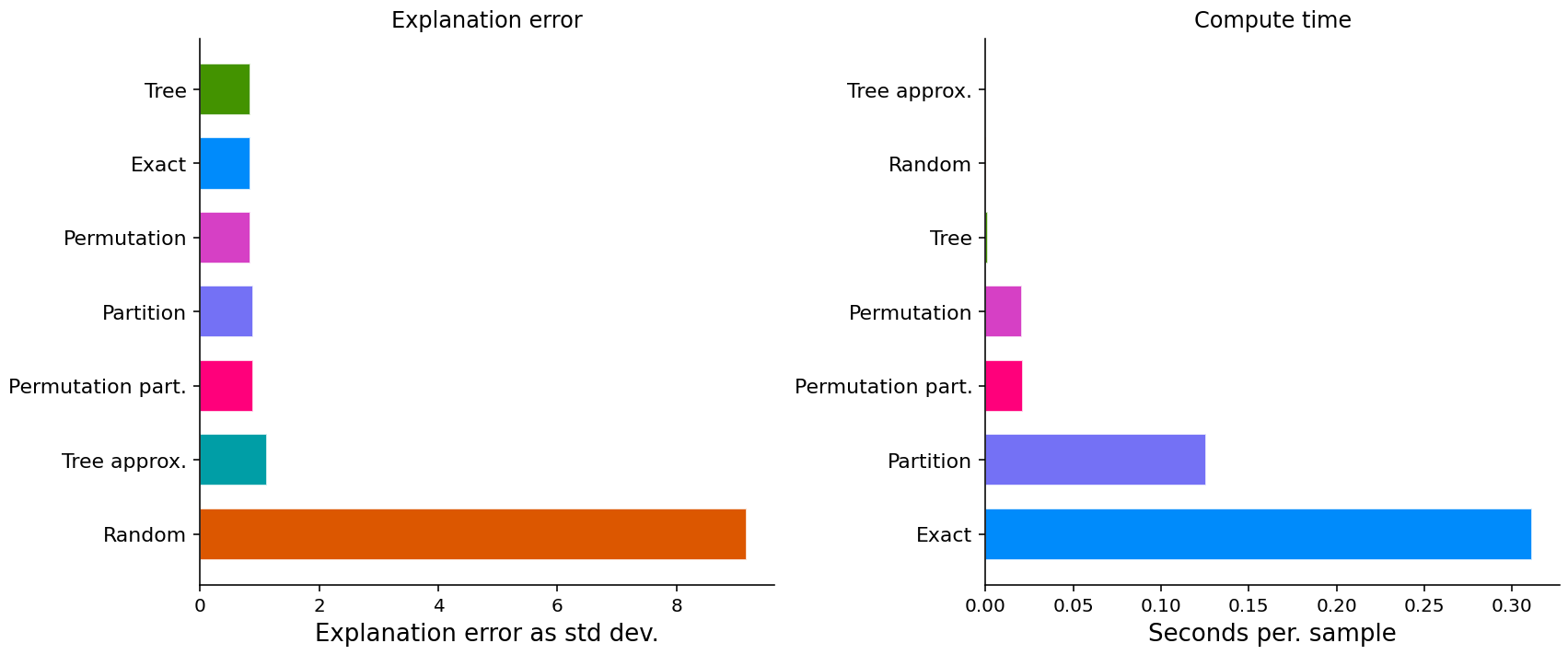
ExplanationError: A measure of the explanation error relative to a model’s actual output.
- For explanations (like Shapley values) that explain the difference between one alternative and another (for example a current sample and typical background feature values) there is possible explanation error for every pattern of mixing foreground and background (i.e., every possible masking pattern).
- compute the standard deviation over these explanation errors where masking patterns are drawn from prefixes of random feature permutations.
- __init__: masker, model, *model_args, batch_size=500, num_permutations=10, link=links.identity, linearize_link=True, seed=38923
- __call__: explanation, name, step_fraction=0.01, indices=[], silent=False

smasker = shap.benchmark.ExplanationError(
    masker, model.predict, X_eval
) # __init__
results["explanation error"] = [smasker(v, name=n) for n,v in attributions] # __call__

ComputeTime

ct = shap.benchmark.ComputeTime()
results["compute time"] = [ct(v, name=n) for n,v in attributions]

SequentialMasker: auc score after feature perturbations
- __init__: mask_type, sort_order, masker, model, *model_args, batch_size=500
- __call__: explanation, name, **kwargs

for mask_type, ordering in [("keep", "positive"), ("remove", "positive"), ("keep", "negative"), ("remove", "negative")]:
    smasker = shap.benchmark.SequentialMasker(
        mask_type, ordering, masker, model.predict, X_eval
    )
    results[mask_type + " " + ordering] = [smasker(v, name=n) for n,v in attributions]

cmasker = shap.maskers.Composite(masker, shap.maskers.Fixed())
for mask_type, ordering in [("keep", "absolute"), ("remove", "absolute")]:
    smasker = shap.benchmark.SequentialMasker(
        mask_type, ordering, cmasker, lambda X, y: (y - model.predict(X))**2, X_eval, y_eval
    )
    results[mask_type + " " + ordering] = [smasker(v, name=n) for n,v in attributions]

Visualize Results

shap.plots.benchmark

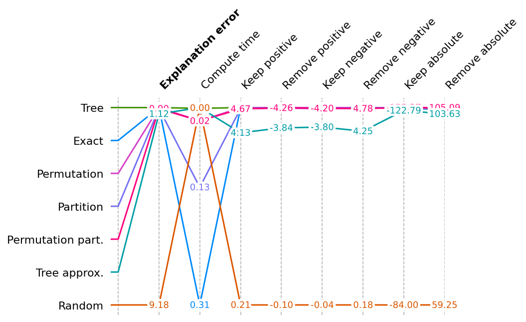
Show scores across all metrics for all explainers

This multi-metric benchmark plot sorts the method by the first method, and rescales the scores to be relative for each metric, so that the best score appears at the top and the worse score at the bottom.

# accept a list of BenchmarkResult 
shap.plots.benchmark(sum(results.values(), []))
# plot without Random
shap.plots.benchmark(filter(lambda x: x.method != 'Random', sum(results.values(), [])))

benchmark_shap

Show detail plots of each metric type

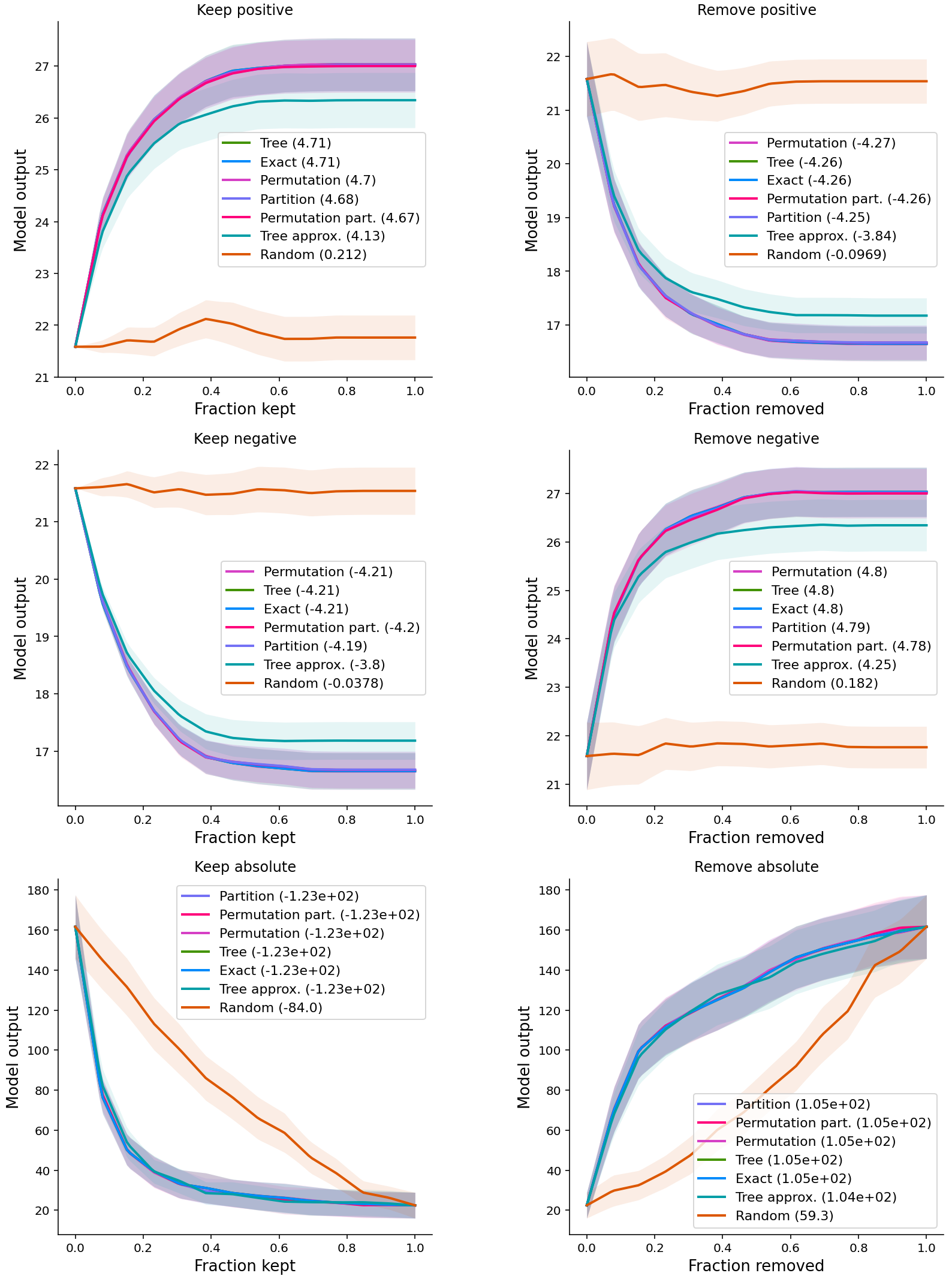
If we plot scores for one metric at a time then we can see a much more detailed comparison of the methods.

import matplotlib.pyplot as plt
num_plot_rows = len(results) // 2 + len(results) % 2
fig, ax = plt.subplots(num_plot_rows, 2, figsize=(12, 5 * num_plot_rows))

for i, k in enumerate(results):
    plt.subplot(num_plot_rows, 2, i+1)
    shap.plots.benchmark(results[k], show=False)
if i % 2 == 0:
    ax[-1, -1].axis('off')
plt.tight_layout()
plt.show()

Some methods just have a score (explanation error and compute time).

Other methods have entire performance curves, and the score is the area under (or over) these curves.

Postive: important features; Negative: unimportant features
For the first two rows, the y-axis of the curves is the original output of XGBoost
For the last row, the output is (y - model.predict(X))**2