
Contents
背景知识 - IG 和 SmoothGrad
Expected gradients combines ideas from Integrated Gradients, SHAP, and SmoothGrad into a single expected value equation.
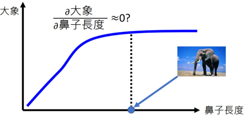
Integrated Gradients (IG)
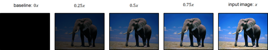
使用梯度的积分来解释模型,可以解决“某特征贡献饱和时梯度为0”的问题,需要一个基线图片(与原图片多次线性插值)来做积分。
SmoothGrad
核心思想是“removing noise by adding noise”,来源于“给图片加微小扰动会造成梯度解释不稳定”的发现,解决方法是“将 n 张扰动图片的梯度平均”。
若将原始的显著图表示 $M(x) = \partial y / \partial x$,则 SmoothGrad 提出的锐化(shapen gradient-based saliency map)方法记作
\[\hat M(x) = \frac{1}{n}\sum_{1}^{n}M(x+\mathcal N(0,\sigma^2))\]实验表明扰动样本越多($n$越大),显著图越稳定。
SHAP源码 - GradientExplainer 类
class Gradient(Explainer):
    """ Explains a model using expected gradients (an extension of integrated gradients).
    Expected gradients an extension of the integrated gradients method (Sundararajan et al. 2017), a feature attribution method designed for differentiable models based on an extension of Shapley values to infinite player games (Aumann-Shapley values). Integrated gradients values are a bit different from SHAP values, and require a single reference value to integrate from.
    As an adaptation to make them approximate SHAP values, expected gradients reformulates the integral as an expectation and combines that expectation with sampling reference values from the background dataset. This leads to a single combined expectation of gradients that converges to attributions that sum to the difference between the expected model output and the current output.
    """
As an adaptation to make them approximate SHAP values, expected gradients reformulates the integral as an expectation and combines that expectation with sampling reference values from the background dataset.
ExpectedGradients
根据 issue #1010 ,GradientExplainer 参考 paper 实现,是IG算法的扩展,通过随机采样插值数量和基线图片来实现,论文中定义的 ExpectedGradients 如下: \(\begin{align} ExpectedGradients_i(x)&:=\int_{x^\prime}IntegratedGradients_i(x,x^\prime)p_D(x^\prime)dx^\prime \\ &= \int_{x^\prime}\left(\left(x-x^\prime\right) \times \int^1_{\alpha=0}\frac{\delta f\left(x^\prime + \alpha \left(x - x^\prime \right)\right)}{\delta x_i} d\alpha \right) p_D(x^\prime)dx^\prime \\ &= \mathop{\mathbb{E}}\limits_{x^\prime \sim D,\alpha \sim U(0,1)}\left[\left(x - x^\prime \right) \times \frac{\delta f\left(x^\prime + \alpha \left(x - x^\prime \right)\right)}{\delta x_i} \right] \end{align}\)
GradientExplainer
阅读源码可知,代码中求期望时结合 SmoothGrad,将 x 扩展为 $x+\Delta, \Delta \sim \mathcal N(0,\sigma^2)$
以下截取 shap_values 方法对应于tensorflow模型的实现
# X ~ self.model_input
# X_data ~ self.data

# samples_input = input to the model
# samples_delta = (x - x') for the input being explained - may be an interim input
期望在 nsamples 个数据样本上求得,三处随机抽取的地方分别关联于变量 rind, t, local_smoothing
"""
class _TFGradient:
function shap_values(self, X, nsamples=200, ...)
"""
samples_input = [np.zeros((nsamples,) + X[l].shape[1:], dtype=np.float32) for l in range(len(X))]
samples_delta = [np.zeros((nsamples,) + X[l].shape[1:], dtype=np.float32) for l in range(len(X))]

for j in range(X[0].shape[0]):
    for k in range(nsamples):
        rind = np.random.choice(self.data[0].shape[0]) # 用于从background dataset(D)中采样baseline input
        t = np.random.uniform() # 插值系数(alpha)
        for l in range(len(X)):
            x = X[l][j] + np.random.randn(*X[l][j].shape) * self.local_smoothing # 对input做smooth,即加高斯噪声(Delta)
            samples_input[l][k] = t * x + (1 - t) * self.data[l][rind]
            samples_delta[l][k] = x - self.data[l][rind]

	# compute the gradients at all the sample points
    find = model_output_ranks[j,i]
    grads = []
    for b in range(0, nsamples, self.batch_size):
        batch = [samples_input[l][b:min(b+self.batch_size,nsamples)] for l in range(len(X))]
        grads.append(self.run(self.gradient(find), self.model_inputs, batch))
    grad = [np.concatenate([g[l] for g in grads], 0) for l in range(len(X))]

	# assign the attributions to the right part of the output arrays
    for l in range(len(X)):
        samples = grad[l] * samples_delta[l]
        phis[l][j] = samples.mean(0)

    output_phis.append(phis[0] if not self.multi_input else phis)
通过 pdb 调试源码可以更快的理解:
import tensorflow as tf
import numpy as np
from shap import GradientExplainer

# model = load_model(...)
dataset = np.random.random([2,20000,18])
explainer = GradientExplainer(model, dataset)
tf_explainer = explainer.explainer

import pdb
dummy_input = np.random.random([1,20000,18])
pdb.run('tf_explainer.shap_values(dummy_input)')
(Pdb) s # 运行当前行,在第一个可以停止的位置(在被调用的函数内部或在当前函数的下一行)停下。
--Call--
> xxx/site-packages/shap/explainers/_gradient.py(199)shap_values()
-> def shap_values(self, X, nsamples=200, ranked_outputs=None, output_rank_order="max", rseed=None, return_variances=False):
(Pdb) unt 302 # 运行到“行号”为止,可以用`l`来查看附近位置的源码
> xxx/site-packages/shap/explainers/_gradient.py(302)shap_values()
-> output_phi_vars.append(phi_vars[0] if not self.multi_input else phi_vars)
(Pdb) len(samples_delta)
1
(Pdb) samples_delta[0].shape
(200, 20000, 18)
(Pdb) grad[0].shape # 200 个采样数据的梯度
(200, 20000, 18)
(Pdb) samples.mean(0).shape
(20000, 18)
示例代码
how the 7th intermediate layer of the VGG16 ImageNet model impacts the output probabilities
# explain how the input to the 7th layer of the model explains the top two classes

# 获得 layer 层的输入
def map2layer(x, layer):
    feed_dict = dict(zip([model.layers[0].input], [preprocess_input(x.copy())]))
    return K.get_session().run(model.layers[layer].input, feed_dict)

e = shap.GradientExplainer(
    (model.layers[7].input, model.layers[-1].output),
    map2layer(X, 7),
    local_smoothing=0 # std dev of smoothing noise
)
shap_values,indexes = e.shap_values(map2layer(to_explain, 7), ranked_outputs=2)
两个重要方法对应的参数如下
-
初始化方法
__init__model- tf.keras.Model
- (input : [tf.Tensor], output : tf.Tensor)
- torch.nn.Module
- a tuple (model, layer), where both are torch.nn.Module objects
data: 能代表训练数据分布的背景数据集- 可选 [, session, batch_size, …]
-
求特征贡献的方法
shap_valuesX: 待解释的数据- 可选 [, nsamples, ranked_outputs, …]