Contents

• SplineCNN: Fast Geometric Deep Learning with Continuous B-Spline Kernels
  • SplineCNN
    • 符号说明
    • 核心思想
    • 卷积运算
      • 局部支持性
      • Closed B-样条
      • 根节点处理
    • GPU算法
  • 实验结果
    • 图像（图）分类
      • Discussion
    • 图节点分类
    • (shape correspondence) 3D配准
      • Discussion

SplineCNN: Fast Geometric Deep Learning with Continuous B-Spline Kernels

SplineCNN

符号说明

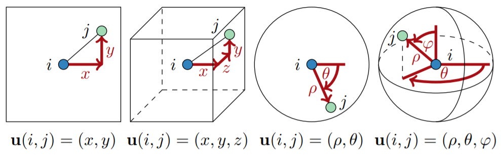
Input graphs.有向图\(G=(V,E,U)\)，其中\(V={1,...,N}\)表示节点集合，\(E\subseteq{V\times{V}}\)表示边集合，\(U\in{[0,1]^{N\times{N}\times{d}}}\)由每条有向边的\(d\)维伪坐标\(u(i,j)\in{[0,1]^d}\)组成；对于一个节点\(i\in{V}\)，它的邻居节点集合表示为\(N(i)\)。

注：伪坐标 (pseudo-coordinates) U的定义是重点，与MoNet论文类似。

U can be interpreted as an adjacency matrix with d-dimensional, normalized entries u(i, j) if (i, j) ∈ E and 0 otherwise

Input node features. 定义映射\(f:V\rightarrow{R^{M_{in}}}\)，其中\(f(i)\in{R^{M_{in}}}\)表示每个节点\(i\in{V}\)的\(M_{in}\)维输入特征的向量。对于\(1\leq{l}\leq{M_{in}}\)，\(f(i)\)中每个特征值的集合\({\{f_l(i)\vert{i\in{V}}\}}\)被称为输入的特征图 (feature map)。

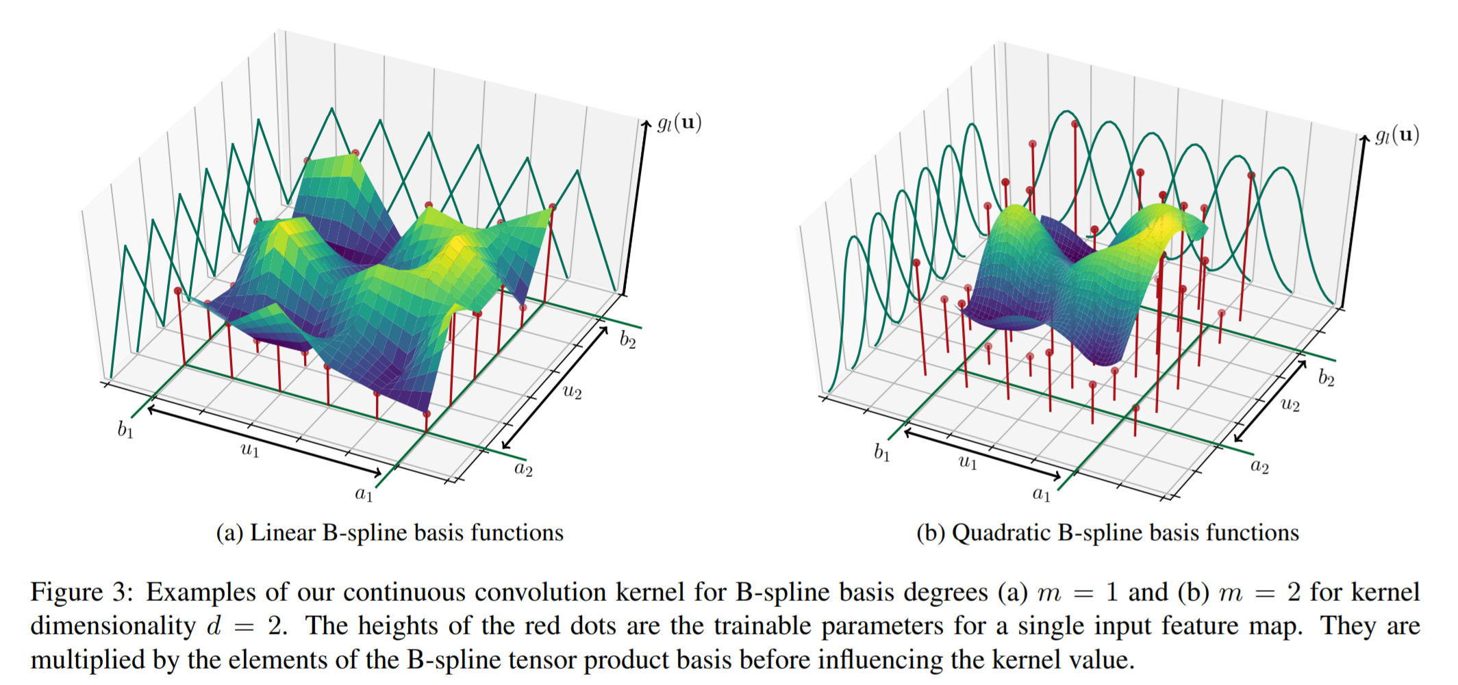
B-spline basis function. \(((N^m_{1,i})_{1\leq{i}\leq{k_1}},...,(N^m_{d,i})_{1\leq{i}\leq{k_d}})\)表示d组\(m\)阶的开(open)B-样条基函数，节点(knots)向量等距分布，即样条均匀(uniform)，其中\(k=(k_1,...,k_d)\)定义了\(d\)维的核大小。

核心思想

特征为\(f(i)\)的节点之间可以是不规则的几何结构，空间关系可以用伪坐标\(U\)来局部定义。在局部聚合邻居特征的时候：\(U\)决定了特征该如何(how)聚合，\(f(i)\)决定了聚合的内容(what)。

常见的几何深度学习任务都可以用此模型表示：

• Graphs: U表示的特征可以是边的权重、节点的度等
• Discrete Manifolds: U可以包含局部的关系信息，如源节点每条边所对应的目标节点的相对极坐标、球坐标或笛卡尔坐标

以下定义了以一个可训练的连续的核函数，加权聚合邻居节点的特征的卷积操作，将每个\(u(i,j)\)映射到一个标量，用作特征聚合时的权重。

卷积运算

• 连续的卷积核函数\(g_l:[a_1,b_1]\times{...}\times{[a_d,b_d]}\rightarrow{R}\)

\[g_l(u)=\sum_{p\in{P}}w_{p,l}\cdot{B_p(u)}\]

​ 其中\(B_p\)是p中所有B-样条基函数的叉乘，即\(B_p(u)=\prod_{i=1}^dN_{i,p_i}^m{u_i}\)，而\(w_{p,l}\)对于每个\(P=((N_{1,i}^m)_i\times{...}\times{(N_{d,i}^m)_i})\)中的元素\(p\)以及特征图中的\(M_{in}\)个值都是可训练的参数，因此可训练的参数总数为\(M_{in}\cdot{K}=M_{in}\cdot{\prod^d_{i=1}}k_i\)。

• 给定核函数集\(g=(g_1,...,g_{M_{in}})\)和输入节点特征\(f\)后，节点\(i\)在空间上的卷积运算可定义为

\[(f*g)(i)=\frac{1}{\vert{N(i)\vert}}\sum_{l=1}^{M_{in}}\sum_{j\in{N(i)}}f_l(j)\cdot{g_l(u(i,j))}\]

局部支持性

由于B-样条基函数的局部支持性，\(B_P\neq0\)只对K个\(p\in{P}\)中的\(s:=(m+1)^d\)个成立。因此对于每个邻居节点\(j\)而言，只依赖于\(M_{in}\times{K}\)中的\(M_{in}\times{s}\)个参数。

一般的，常量s,d,m都是较小的值；另外，给定了m和d之后，对于每对节点\((i,j)\in{E}\)，满足\(B_p\neq0\)的向量\(p\in{P}\)可以在常量时间内被找到，记作\(P(u(i,j))\)，因此之前定义的卷积操作中的每一层还可以写作

\[(f_l*g_l)(i)=\sum_{j\in{N(i)},p\in{P(u(i,j))}}f_l(j)\cdot{w_{p,l}}\cdot{B_p(u(i,j))}\]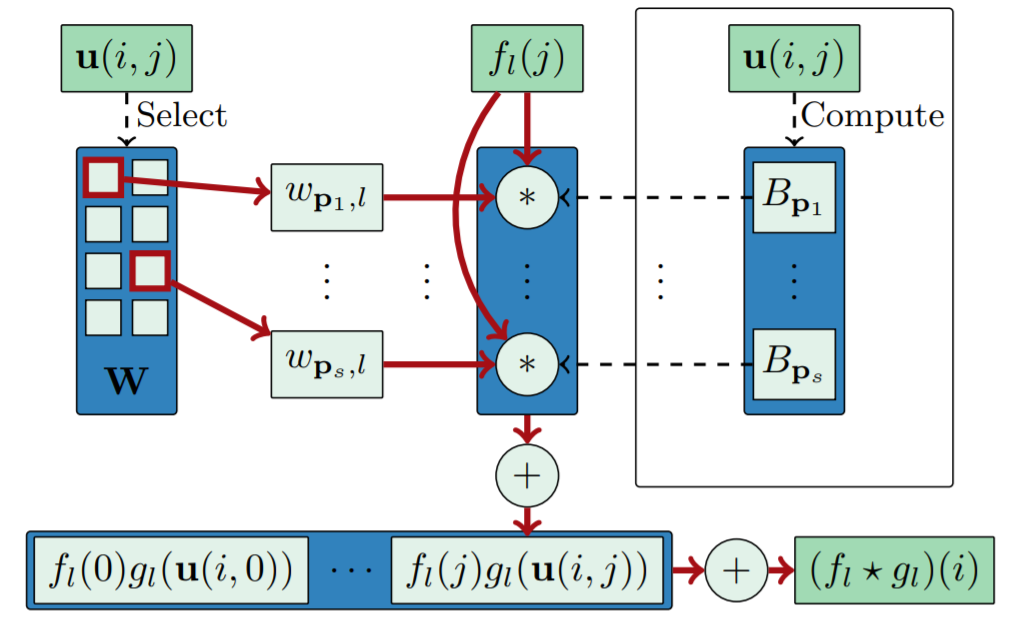

Closed B-样条

根据\(u\)中的坐标轴类型，有时需要选取闭合的B样条估计。例如\(u\)包含极坐标中的角度属性，此时在角度维度使用闭合的B样条估计，可以很自然的使角度为0时和角度为\(2\pi\)时或者更高阶数的情况下权重相同。

要做到这一点，只要通过将某些\(w_{p,l}\)置为周期的，以使核函数\(d\)维中的某些子集维为closed即可。

根节点处理

之前定义的卷积操作聚合了节点\(i\)的邻居节点\(N(i)\)的特征，但没有考虑它自身。如果使用笛卡尔坐标的话，可以很简单的把\(i\)包含到\(N(i)\)中；但对于伪坐标是极坐标/球坐标的情况，半径等于0未被定义。

此时可以为根节点的每个特征引入一个新的可训练的权重，再把它和相应特征的乘积加到结果中去即可。

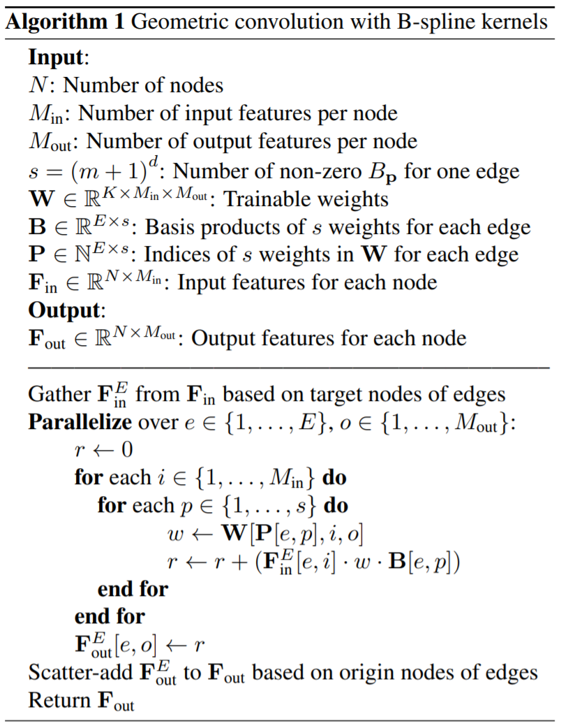
GPU算法

实验结果

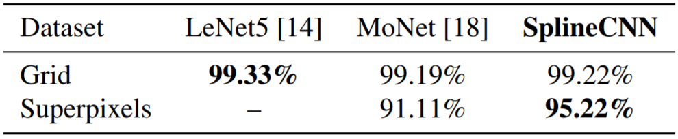
图像（图）分类

[MNIST] 60,000 training and 10,000 test images containing grayscale, handwritten digits from 10 different classes

1. equal grid graphs (\(28\times28\) nodes)

   • LeNet5-like network architecture: \(SConv((5, 5), 1, 32)\rightarrow{MaxP(4)}\rightarrow{SConv((5, 5), 32, 64)} \\ \rightarrow{MaxP(4)}\rightarrow{FC(512)}\rightarrow{FC(10)}\)
   • mirror the LeNet5 architecture with its 5 × 5 filters: neighborhoods of size 5 × 5 from the grid graph
   • reach equivalence to the traditional convolution operator in CNNs: m=1

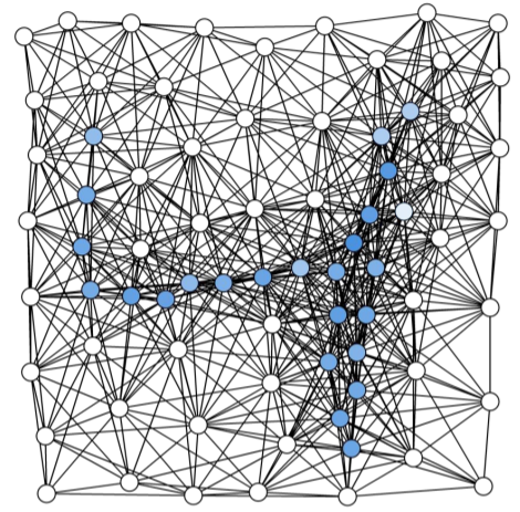
2. embedded graph of 75 nodes defining the centroids of superpixels [超像素]

   [MoNet] F. Monti, D. Boscaini, J. Masci, E. Rodola, J. Svoboda, and M. M. Bronstein. Geometric deep learning on graphs and manifolds using mixture model CNNs. In Proceedings IEEE Conference on Computer Vision and Pattern Recognition (CVPR), pages 5425–5434, 2017.

   ​ \(w_j(u) = exp(−\frac1 2 (u − µ_j )^⊤Σ_j^{−1} (u − µ_j ))\)

   ​ \(Σ_j\) and \(µ_j\) are learnable d × d and d × 1 covariance matrix and mean vector of a Gaussian kernel

   • architecture: \(SConv((k_1,k_2), 1, 32)\rightarrow{MaxP(4)}\rightarrow{SConv((k_1, k_2), 32, 64)} \\ \rightarrow{MaxP(4)}\rightarrow{AvgP}\rightarrow{FC(128)}\rightarrow{FC(10)}\)
   • Cartesian coordinates: \(k_1=k_2=4+m\); Polar coordinates: \(k_1=1+m, k_2=8\)

   

Discussion

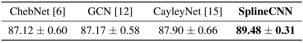
• 实验1中三种方法表现类似

• 实验2中准确率优于MoNet约4.11个百分点：in contrast to the MoNet kernels, our kernel function has individual trainable weights for each combination of input and output feature maps, just like the filters in traditional CNNs.

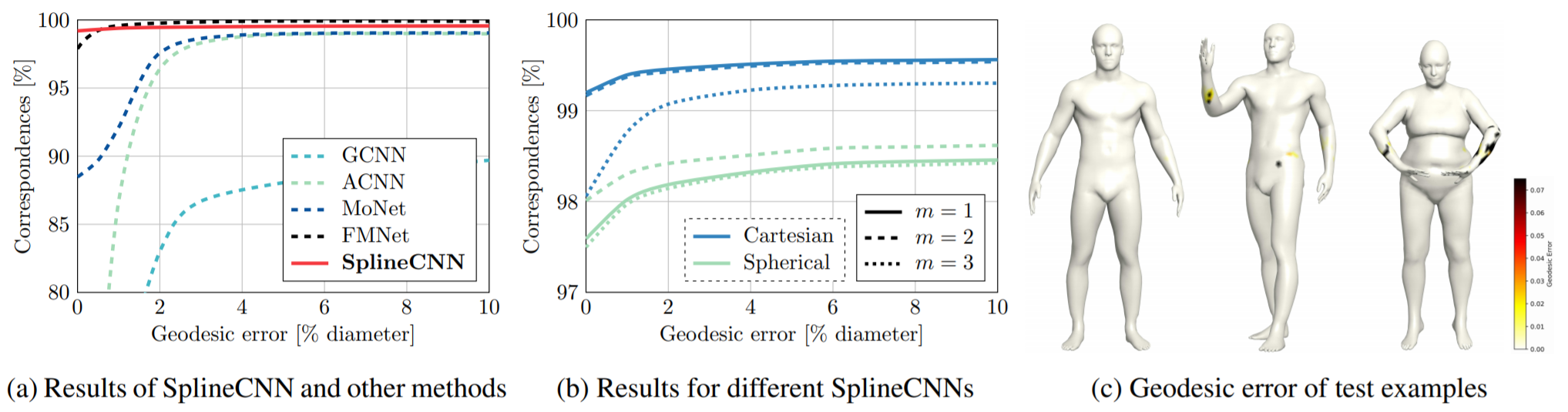
• Different configurations

  

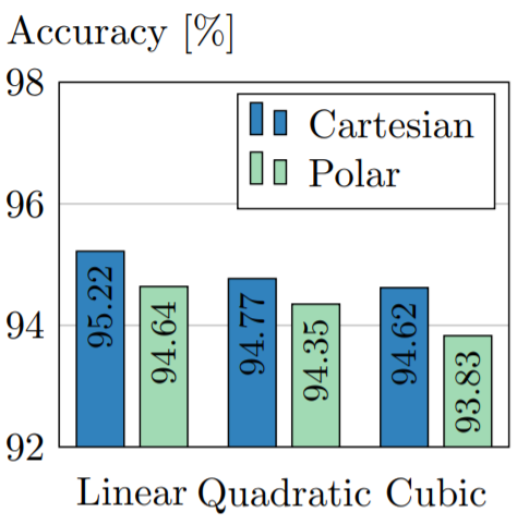
  • 横坐标：阶数m（线性，二次，立方）；图例：两种不同的伪坐标
  • 使用阶数较小的B样条基函数和笛卡尔坐标时的表现略优于其他设置

图节点分类

[Cora] Nodes: 2708 scientific publications (classified into one of seven classes); Links: 5429 undirected unweighted.

Each publication (document) in the dataset is described by a 0/1-valued word vector indicating the absence/presence of the corresponding word from the dictionary (1433 unique words).

• no Euclidean relations
• pseudo-coordinates: globally normalized degree of the target nodes \(u(i, j)=\frac{deg(j)}{max_{v\in{V}}deg(v)}\)
• architecture: \(SConv((2), 1433, 16)\rightarrow{SConv((2), 16, 7)}, m=1\)

(shape correspondence) 3D配准

[FAUST] 100 scanned human shapes in 10 different poses, resulting in a total of 100 non-watertight meshes with 6890 nodes each

[Princeton benchmark protocol] Correspondence quality: counting the percentage of derived correspondences that lie within a geodesic radius r around the correct node.

• three-dimensional meshes

• architecture: \(SConv((k_1, k_2, k_3), 1, 32)\rightarrow{SConv((k_1, k_2, k_3), 32, 64)} \\ \rightarrow{SConv((k_1, k_2, k_3), 64, 64)}\rightarrow{Lin(256)}\rightarrow{Lin(6890)}\)

  其中\(Lin(o)\)表示输出 \(o\) 维特征的\(1\times1\)卷积层

• end-to-end: without handcrafted feature descriptors, input features are trivially given by \(1∈R^{N×1}\)（每个节点的特征都简单地被初始化为1）

Discussion

• [测地距离]错误为0时，匹配率99.2%优于其他所有方法

• 在更大的测地错误边界上的全局表现略低于FMNet，可能的原因是损失函数设置的不同。但值得强调的是，其他方法都使用SHOT特征描述子作为输入（非端到端）。

  While we train against a one-hot binary vector using the cross entropy loss, FMNet trains using a specialized soft error loss, which is a more geometrically meaningful criterion that punishes geodesically far-away predictions stronger than predictions near the correct node